The UK’s productivity puzzle is in the top tail of the distribution

Patrick Schneider

UK productivity growth has been puzzlingly slow since the crisis. After averaging 2% every year in the pre-crisis decade, growth in labour productivity (output per hour worked) has slowed to an average of only 0.5%. Extensive research and commentary on the productivity puzzles has suggested myriad causes for the malaise – including ‘zombie’ firms hoarding resources, sluggish investment in the face of uncertainty, mismeasurement and more – and have dismissed others that no longer seem plausible – including temporary labour hoarding. Using firm-level data, I show that slower aggregate growth is entirely driven by the more productive firms in the economy.

In apparent contrast to my results, recent arguments have focused on the role that the weakest firms play in keeping down aggregate productivity. For example, Andy Haldane highlighted the ‘long tail of low-productivity companies’, which drags on the aggregate, in a speech last year and the OECD has published several papers (e.g. here [pdf] and here) analysing the divergence of the top end of the productivity distribution (‘frontier’ firms) from the rest (‘laggards’).

These ideas have been very influential. But unproductive firms are not responsible for all of the UK’s issues. Using a new method that links aggregate productivity to its distribution across workers, I found that the slowdown in productivity growth is isolated in the top tail of the distribution of productivity across workers. The most productive firms are failing to improve on each other at the same rate as their predecessors did.

You can see this in Chart 1 – the two lines track the average, annual change in productivity at different parts of the distribution across workers, before and after the crisis. The post-crisis line is well below the pre-crisis one, but only toward the right, the top tail of the distribution. Surprisingly, the bottom end of the distribution appears to have been growing faster in recent years than it was leading up to the crisis.

Chart 1: Av. annual change in productivity, by centile of the productivity level distribution

The beauty of this chart is that the average height of each line is about equal to the change in the aggregate – so we can see which part of the distribution is moving (or not) to cause the aggregate to move. And, again, it’s the top end that’s doing the work. This fact doesn’t explain the puzzle. As with any statistical decomposition, we’re brought no closer to the why of the issue, but the where is a little clearer.

That’s about all I have to say. The rest of this post provides the working behind Chart 1. In the next section, I sketch the method I used, and then I take it to UK data, giving a bit more flavour to the result, ending up right back at Chart 1.

One thing this extra detail does is to confirm the headline results in Andy’s speech and the OECD’s papers. You can see the long tail of low productivity firms in Chart 4, and the divergence of the top end of the distribution from the rest in Chart 1. But in the data we have, these features are always there. So they can’t be to blame for the slowdown in growth. Indeed, if anything, the increasing dispersion is where aggregate growth usually comes from. In this light, the UK growth puzzle is there because the increasing dispersion has slowed down since the crisis.

The method (for the interested reader)

So how did I get to Chart 1?

Aggregate labour-productivity (value-added per worker) is usually measured by taking a labour-weighted average of firm-level productivity.  But it can also be approximated by the average of a number (Q) of equally spaced quantiles (as I outline in a forthcoming working paper). So, for example, we could measure aggregate productivity by taking the average of the 1^st through 99^th centiles of the distribution. More explicitly

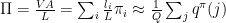
where and represent firms and quantiles, is productivity, is value-added and is labour. is the quantile function of productivity across workers, it picks out the productivity of the worker who is more productive than exactly of the others.

(Aside: we need to be careful to work with the correct distribution. The key is that aggregate productivity is the mean of the distribution across workers. Because we usually measure productivity at the firm level, we need to use labour weights to adjust the calculation to the right distribution.)

With this approximation, we can measure changes in the aggregate by averaging over changes in the centiles as well. Using the formula below, we can see which part of the distribution is moving (or not) to cause the aggregate to move.

Note that we’re tracking growth in the distribution here – not growth in firms, nor the distribution of firm growth, so it could be that parts of the distribution move around or stay still, but the firms that are located there are shifting around a lot.

The data (for the still interested reader)

So now that we have the method in hand, let’s apply it to UK data.

I’m using ONS firm-level microdata (combining ARDx with ABS 2015), and measuring productivity as real value-added (using 2-digit sector deflators) per employee.

This dataset doesn’t cover the whole economy – the surveys only try to cover the non-financial business economy (which is a shame given the importance of finance in the growth puzzle) and some other sectors only pop up from 2009, so I had to cut these from the whole dataset for consistency. Because of these survey limitations, the ‘aggregate’ in the below results is a subset of the overall UK aggregate economy.

OK so let’s first check how close the approximation is. The charts below show actual productivity and its growth as measured from the micro-data, compared with the approximation. As you can see in Chart 2, the approximation has a consistent negative bias, because cutting out the top 1% drops some very large outliers, but the growth path is about right (Chart 3).

Chart 2: Aggregate productivity and its centile approximation (level)

Chart 3: Aggregate productivity and its centile approximation (growth)

 

Now that we know the approximation matches the aggregate patterns pretty well, we can look at the distributions underlying these aggregate figures. And we find:

1. The productivity distribution is highly skewed (chart 4), so the top tail has a very strong influence on the aggregate.

The distribution has a long tail of workers in unproductive firms at the bottom, and workers in a collection of the ‘happy few’ extremely productive firms at the top. This is a well-known feature of the productivity distribution, regardless of whether we weight by labour or not. An implication of this shape is that the top tail has a very strong influence on the level of aggregate productivity in any given year, just as large outliers will push up on any average.

Chart 4: Most of the distribution is stable over time

2. The top tail has an even greater influence on changes in aggregate productivity from year to year.

Over 70% of the growth in aggregate productivity between 2003 and 2015 was driven by the top two deciles.  This is because the rest of the distribution doesn’t move around much; at least not in magnitudes that compare to movements in the upper tail (chart 4). Incidentally, this is the same thing as the OECD’s observation that the top tail is diverging from the rest.

3. The productivity puzzle (slower aggregate growth after the crisis than before) is located in the top tail of the distribution.

We can locate the growth puzzle by comparing changes in the pre- and post-crisis periods. Chart 5 is a reproduction of chart 1 with an extra line; it shows the average annual change of each centile over three distinct periods – the pre-crisis years (2004-07), the crisis (2008-09) and the post-crisis period (2010-15).

To read the chart, pick a centile and the three lines show how that part of the distribution changed, on average, over these different periods. For example, the median grew at about the same rate pre- and post-crisis, and had quite a drop during the crisis.

Chart 5: Average annual change in productivity by centile

The growth puzzle is the gap between the pre- and post-crisis lines. The chart shows that lower sections of the distribution have actually grown faster post-crisis than they did before it (pink line above the navy) and so cannot be driving the puzzle. By contrast, the top two deciles grew far slower (pink line below the navy) and therefore this is where the growth puzzle is located.

This work contains statistical data from ONS which is Crown Copyright. The use of the ONS statistical data in this work does not imply the endorsement of the ONS in relation to the interpretation or analysis of the statistical data. This work uses research datasets which may not exactly reproduce National Statistics aggregates.

Update 13/08/2018: The Bank Staff Working Paper mentioned above – Schneider (2018) ‘Decomposing differences in productivity distributions’ is now available here.

Patrick Schneider works in the Bank’s Structural Economic Analysis Division.

If you want to get in touch, please email us at bankunderground@bankofengland.co.uk or leave a comment below.

Comments will only appear once approved by a moderator, and are only published where a full name is supplied.Bank Underground is a blog for Bank of England staff to share views that challenge – or support – prevailing policy orthodoxies. The views expressed here are those of the authors, and are not necessarily those of the Bank of England, or its policy committees.